Tutorial 2 of 6
Oscilloscope & function generator
Beginner 10 min
Drive an RC low-pass filter with a square wave and a sine, measure the time constant and the corner frequency on the 4-channel oscilloscope.
This tutorial uses the RC low-pass filter + Bode template: R1 = 1 kΩ, C1 = 100 nF, so the time constant is τ = RC = 100 µs and the corner frequency is f = 1/(2πRC) ≈ 1.59 kHz. Open it from the start screen (Ctrl+N).
There are two ways to watch signals over time:
Transient analysis (F5) | Live mode (F6, Power) | |
|---|---|---|
| What it does | Simulates a fixed stretch of time (e.g. 4 ms) as fast as possible | Simulates continuously at an adjustable speed (e.g. 1 ms of circuit time per second) |
| Good for | Exact measurements, CSV export, the time scrubber | Turning knobs and flipping switches while you watch |
| Instruments | Oscilloscope, results, scrubber | Oscilloscope, multimeter, generator, supply panels |
1. Step response with a pulse source
- Click V1. In the inspector, set Waveform to Pulse with V1 = 0, V2 = 5, width 1 ms and period 2 ms.
- In the toolbar's analysis selector, choose Transient. Under Analysis settings…, set the stop time to
4m. - Open the Oscilloscope tab and set CH1 to IN and CH2 to OUT. You can also click a wire with the probe tool (
P), which adds its net to the next free channel. - Press Run (
F5).
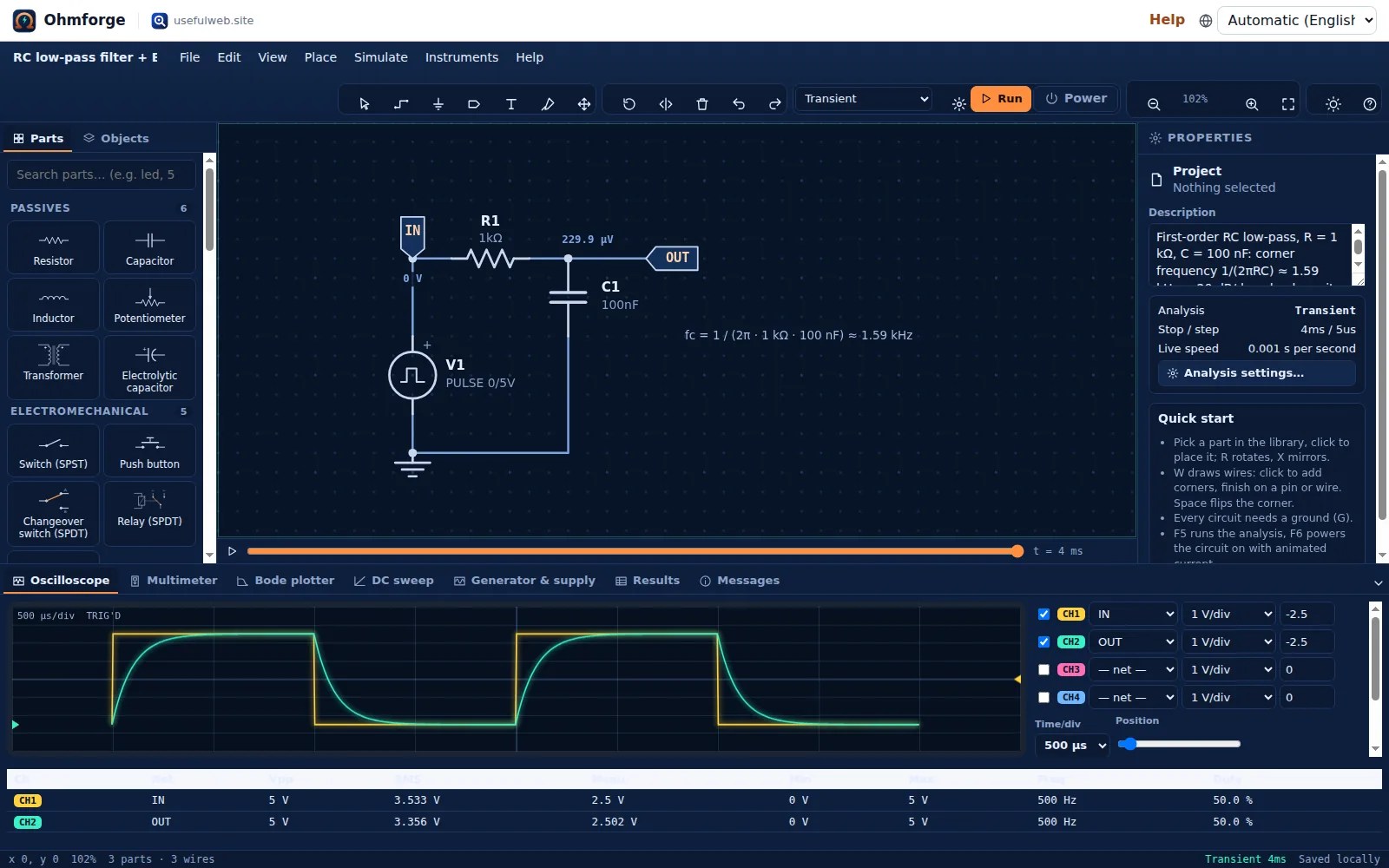
The output rises along 1 − e^(−t/τ). After one time constant (100 µs) it should be at 63.2 % of 5 V, which is 3.16 V. The engine's own transient tool gives 3.152 V at t = 100 µs. You can get the same number from the API (see tutorial 6):
{ "netlist": "* RC step\nV1 in 0 PULSE(0 5 0 1u 1u 1m 2m)\nR1 in out 1k\nC1 out 0 100n\n.tran 10u 2m\n.end", "probes": ["out"], "tstep": 0.0001 }"time": [0, 0.0001, 0.0002, 0.0003, 0.0004, 0.0005, …],
"waveforms": { "out": [0, 3.15195, 4.31926, 4.75018, 4.90919, 4.9665, …] }The 10–90 % rise time comes out as riseTime: 0.000226 s, matching the theory of 2.2 τ = 220 µs.
Drag the orange time scrubber under the schematic to step through the result. The voltage tags and the wire colours follow the scrubber.
Reading the scope
- Time/div and Position set the horizontal axis. Each channel has its own V/div and offset.
- Trigger chooses the source channel, the level and the edge, plus auto/normal/single mode. A stable display of a periodic signal needs the trigger.
- Autoset picks the scales for you. Cursors adds two vertical cursors that show Δt and 1/Δt. CSV exports what's on screen.
- The table under the screen measures every channel: Vpp, RMS, mean, min/max, frequency and duty cycle.
2. A sine at the corner frequency
Set V1 back to Sine with amplitude 1 V and frequency 1.59k, set the stop time to 3m, then run.
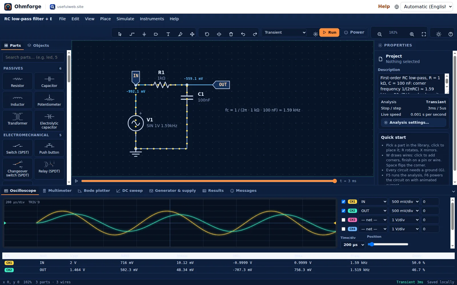
In theory the output at the corner is 1/√2 of the input (−3 dB) and lags by 45°. The scope measures IN 2 V pp and OUT 1.464 V pp. The output is a little above the theoretical 1.414 V because the 3 ms window includes the first cycle, while the capacitor is still charging from zero. Move Position to the last millisecond and the ratio settles at ≈ 0.71. Tutorial 3 shows how to measure frequency response properly, without start-up transients.
3. Use the function generator instead
A plain source is fine for an analysis. For hands-on work there's a Function generator (Instruments category in the library, or Instruments → Place function generator). It has a 50 Ω output and offers sine, square, triangle or saw waves.
Replace V1 with a function generator: set it to square, 500 Hz, amplitude 2.5 V, offset 2.5 V. Then press Power (F6) and open Generator & supply. This panel is the generator's front panel: change the waveform, frequency or amplitude while the circuit runs and watch the scope respond.
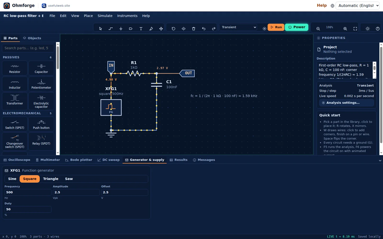
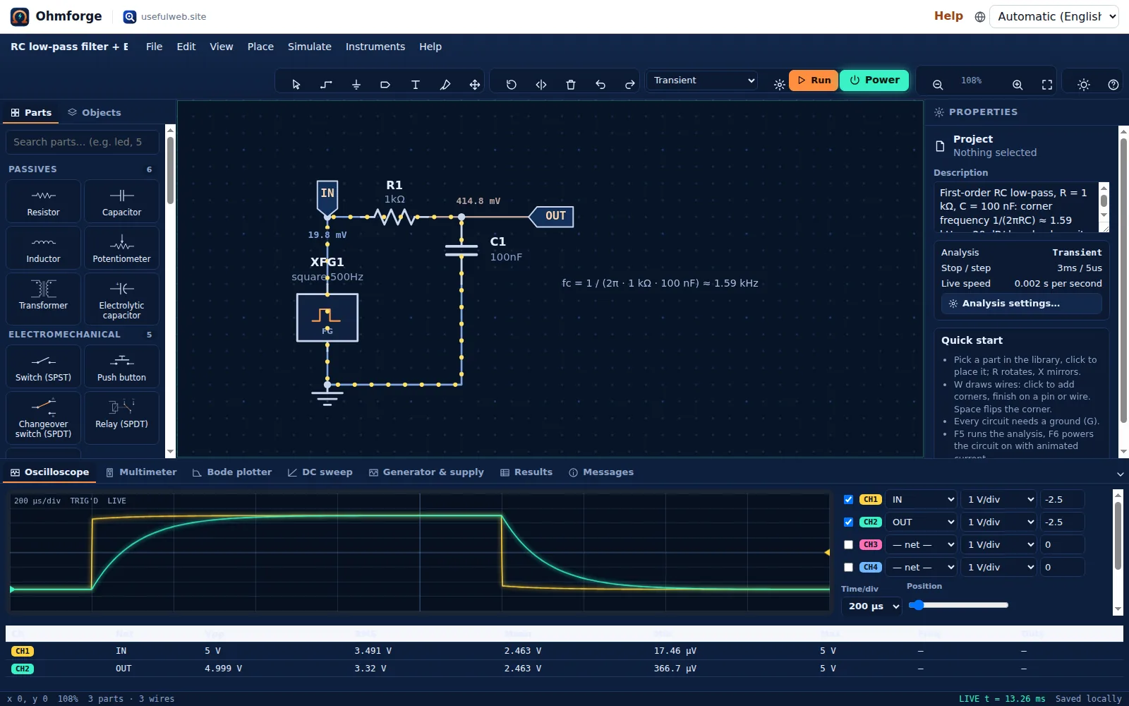
The scope header says LIVE, and Stop freezes the trace. In live mode you set the speed with Analysis settings… → Simulated time per real second. 1 s/s suits blinkers. Audio-frequency circuits like this one need 1–2 ms/s, or the waves pass too fast to see.
Tips
- An empty channel shows "— net —". Probe (
P) a wire to fill the next free channel. - To measure a signal relative to something other than ground, use the multimeter's second probe or the Bode plotter's reference node.
- The CSV button exports the waveforms, so you can compare them with real scope captures in a spreadsheet.
Next: Bode plots and filters