Bode plots and filters

A Bode plot shows how a circuit treats each frequency: the magnitude (gain in dB) and the phase (in degrees) of the output relative to the input. Ohmforge computes it with a small-signal AC sweep. It linearises the circuit around its DC operating point and then solves complex nodal equations at every frequency. Because the sweep starts from a steady state, it has none of the start-up transients you saw on the scope in tutorial 2.

1. The RC low-pass

Open the RC low-pass filter + Bode template and choose the Bode plotter tab:

• Input source: V1. During the sweep it gets an AC magnitude of 1 V, and all other sources become AC-quiet.
• Output net: OUT.
• Relative to: source (1 V). You can pick a node here instead, to get V(out)/V(node).
• From / To / Points/dec: 10 Hz … 1 MHz, 30 points per decade.

Press Sweep.

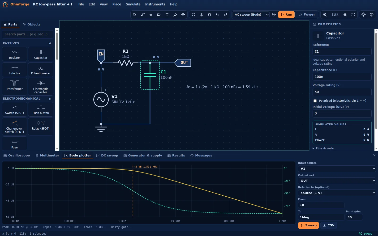
The status line under the plot reads:

Peak -0.00 dB @ 10 Hz · upper −3 dB 1.591 kHz · lower −3 dB — · unity gain —

That matches 1/(2π · 1 kΩ · 100 nF) = 1.5915 kHz. Above the corner, the magnitude falls by 20 dB per decade, which is typical of a first-order filter. At the corner the phase is −45°, and it approaches −90° at high frequencies (the dashed curve, right-hand axis).

The plotter interpolates between sweep points to find the −3 dB frequency, so more points per decade give a more exact corner. The same sweep over MCP with 10 points/decade gives 1.597 kHz, while 20 points/decade give 1.591 kHz.

Try it

• Change C1 to 10n and sweep again. The corner moves up by a factor of ten, to about 15.9 kHz.
• Swap R1 and C1 to get a high-pass filter. The plotter then reports a lower −3 dB frequency instead.
• Press CSV to export frequency, magnitude and phase.

2. An op-amp's bandwidth

Open Non-inverting amplifier. It uses a real op-amp model (TL071-like): finite open-loop gain, 3 MHz gain-bandwidth product, supply rails at ±12 V and output headroom. R1 = 1 kΩ and R2 = 10 kΩ set the gain to 1 + R2/R1 = 11.

Sweep from 10 Hz to 10 MHz with V1 as the input and OUT as the output:

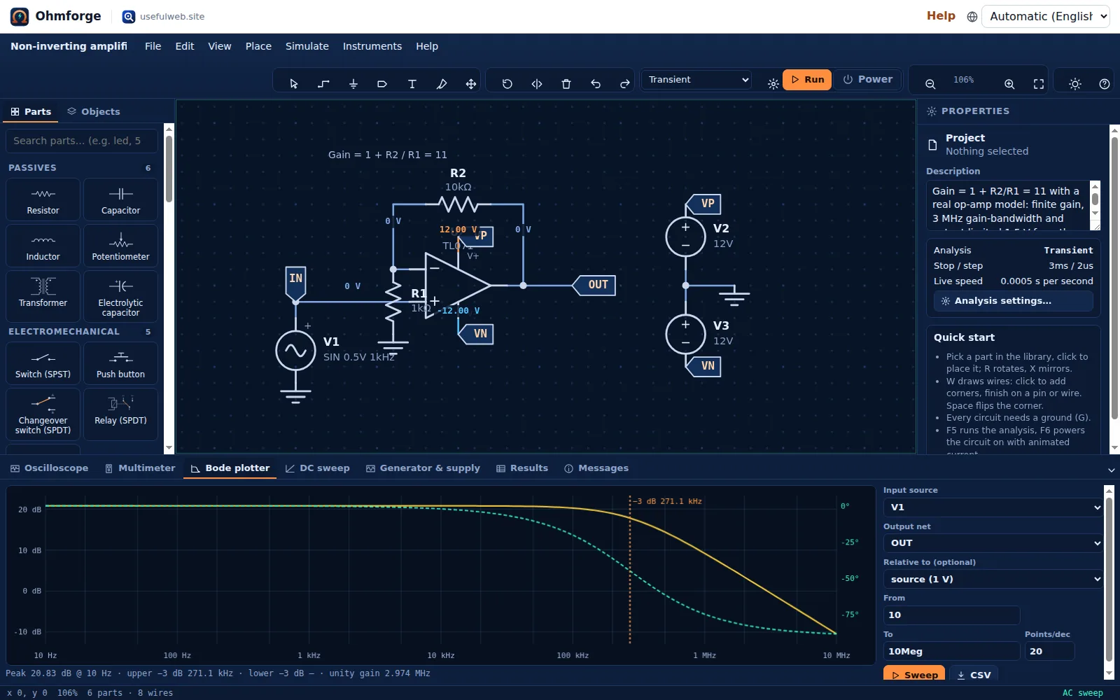
Peak 20.83 dB @ 10 Hz · upper −3 dB 271.1 kHz · lower −3 dB — · unity gain 2.974 MHz

• 20 · log₁₀(11) = 20.83 dB. That is exactly the ideal gain.
• The closed-loop bandwidth is GBW / gain = 3 MHz / 11 ≈ 272.7 kHz, and the plot shows 271.1 kHz.
• Gain falls to 0 dB (unity) near the 3 MHz GBW, as the single-pole model predicts.

Click U1 and raise Gain-bandwidth product in the inspector, or lower the gain by making R2 smaller, and the corner moves accordingly.

Ohmforge offers two op-amp parts. The plain Op-amp (ideal) has a fixed huge gain and no supply pins, which is ideal for learning the textbook rules (its Bode plot is flat). Op-amp (real, with supplies) adds GBW, rails and output limits, so it clips and rolls off like a real chip.

3. Large-signal vs. small-signal

An AC sweep is linear, so it can't show clipping. Set V1's amplitude to 2 V in the non-inverting amplifier: 2 V × 11 = 22 V is above the ±12 V supply. Then compare:

• The Bode plot still says 20.83 dB, because the small-signal gain doesn't change.
• A transient run (F5 in Transient mode) shows the output flattening at ±10.45 V. The model's output stops 1.5 V short of each rail.

The AC tool states the same limit among its assumptions: "Small-signal (linear) analysis around the DC operating point: large-signal effects such as clipping do not appear."

4. DC sweep for transfer curves

The DC sweep tab steps a DC source over a range and plots one net, for example an amplifier's input-to-output transfer curve or a diode's I–V characteristic. You choose Source, Start, Stop, Step and Plot net. For an amplifier, the slope of the curve is the gain, and the flat ends show where the output clips.

Next: Transistors, op-amps and the 555